Search & Ranking Systems: A Practical Guide for Data Scientists

Query understanding, semantic search, learning-to-rank, personalization, transformers, two-tower architectures, LLM ontologies, evaluation — plus a runnable demo.

Search and ranking power discovery in almost every digital product we use: ecommerce, content, jobs, maps, support, and more.

This post is a technical, hands‑on introduction to the main building blocks of search and ranking systems. We’ll look at:

• Query understanding

• Semantic search

• Spell correction

• Ranking / Learning-to-Rank

• Personalization

• Transformer architectures

• Two-tower architectures

• LLM-based ontologies

• Evaluating search results at scale

The goal is that by the end, you’ll know what each concept means and how it fits into a production stack.

---

1. Big Picture: How Modern Search Systems Work

Let’s start with the mental model.

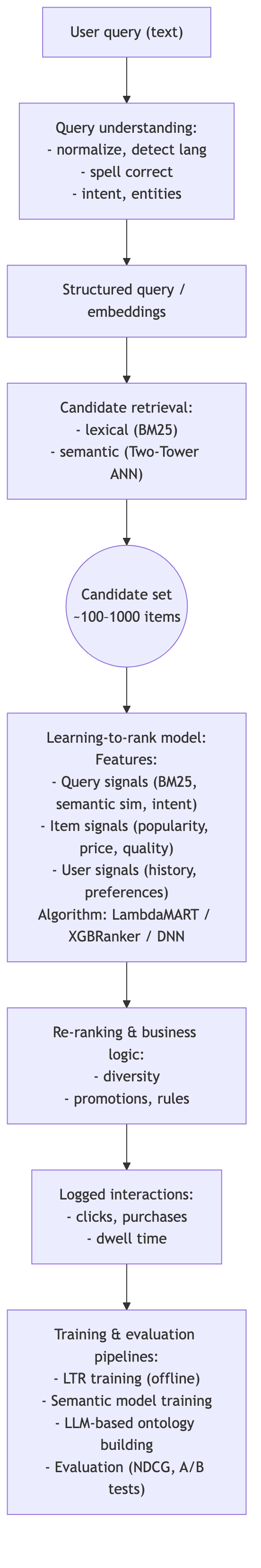
When a user types a query (“sushi”) into a search box, a typical production system looks like this:

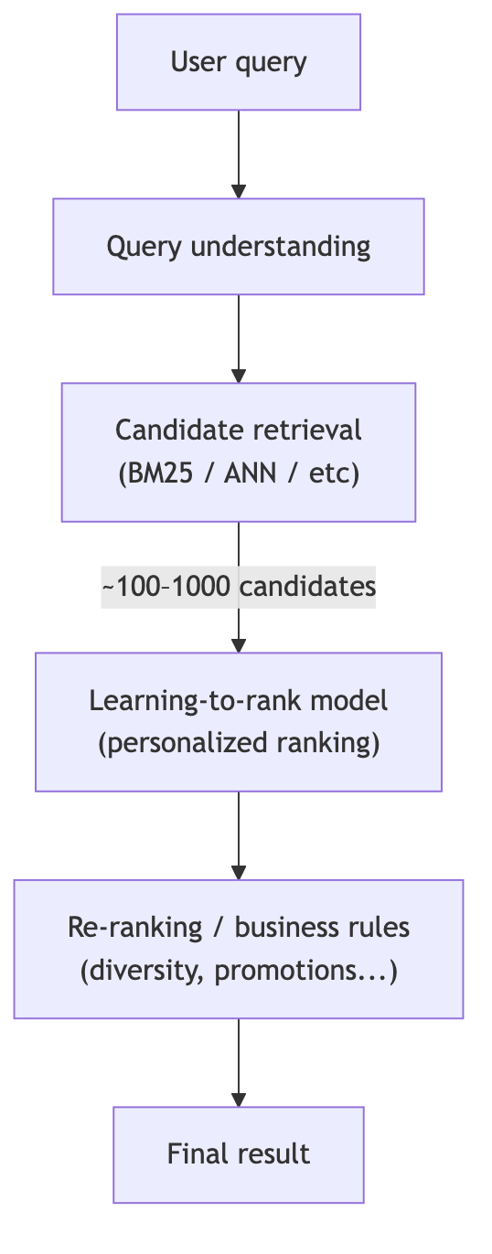
Each block maps to the buzzwords:

• Query understanding: clean and interpret the text (“susshi” → “sushi”, detect intent, extract entities).

• Semantic search & Two‑Tower architectures: retrieve candidates by meaning, not just exact keywords.

• Learning‑to‑Rank: order candidates using ML based on relevance signals.

• Personalization: adjust ranking per user.

• Transformers & NLP: power semantic understanding, embeddings, and generative components.

• LLM‑based ontologies: structure the catalog & concepts to make search smarter.

• Evaluation at scale: measure all of this with offline metrics and online A/B tests.

We’ll go through these components with code and simple architecture diagrams.

---

2. Learning‑to‑Rank (LTR): The Core of Ranking

2.1 Problem setup

In many supervised ML setups you predict one label per row.

In Learning‑to‑Rank, you care about ordering documents for a query:

• Input: query q and documents d₁, …, dₙ

• Features: x_i = f(q, d_i, user, context)

• Output: scores s_i that induce a ranking

Data is grouped by query:

 Query q1:  d1, d2, d3  → label: [2, 0, 1] (relevance levels)
 Query q2:  d4, d5      → label: [0, 1]
 ...

2.2 Three main LTR paradigms

1. Pointwise
   Treat each (q, d) as an independent sample.
   Example: regression on a relevance score (0–3) or classification (clicked / not).

2. Pairwise
   Learn from pairs of documents for the same query.
   For each pair (d+, d−): model learns score(d+) > score(d−).

3. Listwise
   Optimize over the whole ranked list (e.g. approximating NDCG).

In practice, gradient-boosted trees (LambdaMART, XGBoost ranker, LightGBM ranker) are very common in industry because they perform well, are relatively fast, and handle heterogeneous features nicely.

2.3 Minimal LTR example with XGBoost

Below is a toy example using XGBRanker to rank results for different queries.

 import numpy as np
 from xgboost import XGBRanker
 ​
 # Toy data: 3 queries, each with some candidate items
 # Features could be: [BM25_score, semantic_similarity, popularity]
 X = np.array([
     [2.1, 0.4, 10],  # q1-d1
     [1.2, 0.7, 30],  # q1-d2
     [0.5, 0.2,  5],  # q1-d3
     [0.1, 0.9, 50],  # q2-d4
     [0.3, 0.3, 20],  # q2-d5
     [1.0, 0.1,  1],  # q3-d6
     [0.9, 0.6, 15],  # q3-d7
 ])
 ​
 # Relevance labels (higher = more relevant)
 y = np.array([
     2,  # q1-d1
     3,  # q1-d2
     0,  # q1-d3
     3,  # q2-d4
     1,  # q2-d5
     0,  # q3-d6
     2,  # q3-d7
 ])
 ​
 # Group size: number of documents per query
 group = [3, 2, 2]  # q1 has 3 docs, q2 has 2, q3 has 2
 ​
 model = XGBRanker(
     objective=”rank:pairwise”,
     n_estimators=100,
     learning_rate=0.1,
     max_depth=4,
     subsample=0.8,
     colsample_bytree=0.8
 )
 ​
 model.fit(X, y, group=group)
 ​
 # Predict and see the ranking for query 1 documents
 scores_q1 = model.predict(X[0:3])
 ranking_q1 = np.argsort(-scores_q1)  # descending
 print(”Scores q1:”, scores_q1)
 print(”Ranking q1 (indices):”, ranking_q1)

In a real system:

• X is built from many features: lexical, semantic, user, item, context.

• y often comes from logs (clicks, purchases) with some preprocessing.

• group is derived from query IDs.

This is the backbone ranking block in the earlier pipeline diagram.

---

3. Query Understanding

Query understanding is about turning raw user text into something the system can reason about.

Typical sub-tasks:

1. Normalization

   • Lowercasing, Unicode normalization, removing punctuation.

   • Handling accents (“papá” → “papa”), transliteration.

2. Tokenization

   • Split into tokens, handle multi‑word entities (“ice cream”).

3. Spell correction / typo handling

   • “suhshi” → “sushi”.

   • “iphon 15” → “iphone 15”.

4. Intent classification

   • Is the user searching for a product, a category, a help article?

   • Example labels: {”product_search”, “faq_search”, “navigation”, ...}

5. Entity extraction

   • Extract “sushi”, “Amsterdam”, “vegan”, etc.

   • Map to catalog entities: category IDs, locations, cuisines…

6. Query rewriting / expansion

   • Add synonyms, canonicalize terms (“veggie” → “vegetarian”).

3.1 Minimal intent classification example

You can treat query intent classification as a standard text classification problem:

 import numpy as np
 from sklearn.pipeline import Pipeline
 from sklearn.feature_extraction.text import TfidfVectorizer
 from sklearn.linear_model import LogisticRegression
 ​
 queries = [
     “iphone 15 pro max”,
     “refund policy”,
     “restaurants near me”,
     “track my order”,
     “vegan sushi”,
 ]
 ​
 labels = [
     “product_search”,
     “faq_search”,
     “local_search”,
     “faq_search”,
     “product_search”,
 ]
 ​
 pipe = Pipeline([
     (”tfidf”, TfidfVectorizer(ngram_range=(1, 2))),
     (”clf”, LogisticRegression(max_iter=1000)),
 ])
 ​
 pipe.fit(queries, labels)
 ​
 print(pipe.predict([”cancellation policy”]))
 print(pipe.predict([”best burgers in berlin”]))

In production, you’d likely use:

• Better tokenization (e.g. spaCy, HuggingFace tokenizers)

• Possibly a transformer encoder (see next sections)

• More sophisticated labels and training data

---

4. Semantic Search & Two‑Tower Architectures

4.1 Lexical vs semantic search

Traditional search (BM25, TF‑IDF) is lexical:

• Relevance is based on overlap of terms between query and document.

• “cheap phone” won’t match “affordable smartphone” very well.

Semantic search uses vector representations (embeddings) of text:

• Encode queries and documents into vectors in ℝᵈ.

• Similar meanings → close in vector space (via cosine / dot product).

• Retrieval: find top‑K documents with highest similarity.

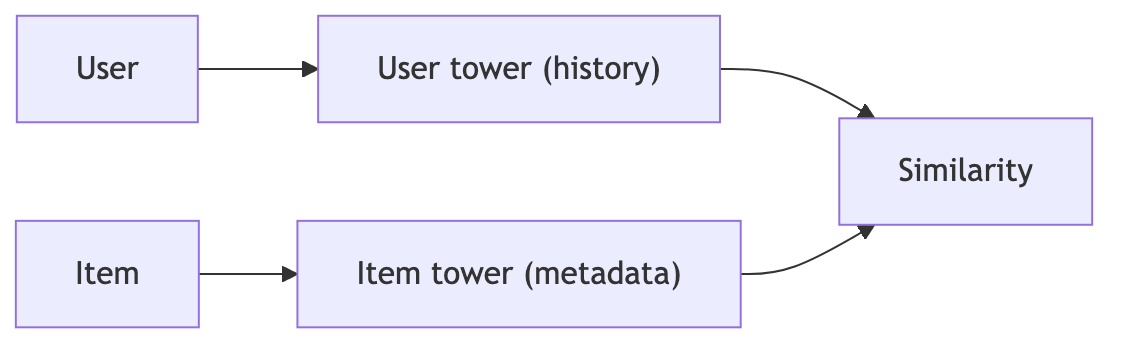
4.2 Two‑Tower (Dual-Encoder) architecture

For scalable semantic retrieval, a common pattern is the Two‑Tower architecture:

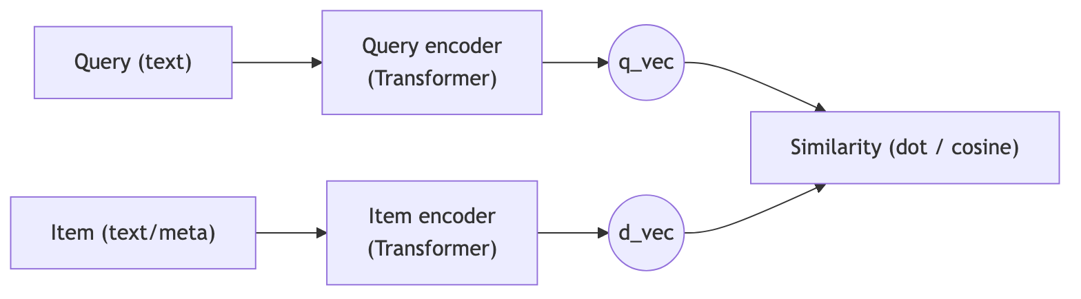
• The query encoder and item encoder share architecture but may (or may not) share weights.

• You pre-compute and index item embeddings in an ANN index (FAISS, ScaNN, etc).

• At query time, compute q_vec, then retrieve top‑K items by similarity.

4.3 Training objective (contrastive learning)

Given training triples (q, d⁺, d⁻) where d⁺ is relevant and d⁻ is not, you can train with a contrastive loss.

Pseudo‑code:

 import torch
 import torch.nn as nn
 import torch.nn.functional as F
 ​
 class DualEncoder(nn.Module):
     def __init__(self, text_encoder):
         super().__init__()
         self.query_encoder = text_encoder()
         self.doc_encoder = text_encoder()
 ​
     def encode_query(self, queries):
         return self.query_encoder(queries)  # [batch, dim]
 ​
     def encode_doc(self, docs):
         return self.doc_encoder(docs)      # [batch, dim]
 ​
 def contrastive_loss(q_vecs, d_pos_vecs, d_neg_vecs, temperature=0.05):
     # q_vecs, d_pos_vecs, d_neg_vecs: [batch, dim]
     # Construct logits: [batch, 1 + num_neg]
     pos_scores = (q_vecs * d_pos_vecs).sum(dim=-1, keepdim=True)  # [B,1]
     neg_scores = (q_vecs.unsqueeze(1) * d_neg_vecs).sum(dim=-1)   # [B, num_neg]
 ​
     logits = torch.cat([pos_scores, neg_scores], dim=1) / temperature
     labels = torch.zeros(q_vecs.size(0), dtype=torch.long)  # index 0 is positive
 ​
     return F.cross_entropy(logits, labels)

In practice you’d use a real transformer encoder (e.g., BERT-like model), proper batching, and possibly in-batch negatives (each positive is a negative for others).

4.4 Simple semantic search example with pre-trained model

If you don’t want to train from scratch, you can use existing sentence embedding models:

 from sentence_transformers import SentenceTransformer, util
 ​
 model = SentenceTransformer(”all-MiniLM-L6-v2”)
 ​
 documents = [
     “Cheap smartphone with good battery life”,
     “Italian restaurant with vegan options”,
     “Used car marketplace”,
 ]
 doc_emb = model.encode(documents, convert_to_tensor=True)
 ​
 query = “affordable phone with long battery”
 q_emb = model.encode(query, convert_to_tensor=True)
 ​
 cos_scores = util.cos_sim(q_emb, doc_emb)[0]
 top_k = cos_scores.topk(k=3)
 for score, idx in zip(top_k.values, top_k.indices):
     print(float(score), documents[int(idx)])

This is a semantic retrieval layer that can feed candidates into your LTR model.

---

5. Transformer Architecture: Why It Shows Up Everywhere

Transformers underpin much of modern NLP, including semantic search, query understanding, and LLMs.

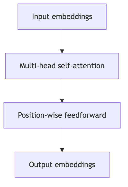
5.1 Core ideas

• Input sequence is tokenized into tokens t₁, …, tₙ.

• Each token mapped to an embedding, plus positional encodings.

• Multiple layers of self‑attention + feed‑forward networks.

• Self‑attention lets each token attend to all others in the sequence.

Simplified encoder block:

Encoder‑only models (BERT, RoBERTa):

• Great for classification, retrieval, sentence embeddings.

• Often used as the backbone in query/item encoders.

Decoder‑only / LLMs (GPT‑like):

• Great for generative tasks: query rewriting, summarization, plan generation, ontology induction (later section).

You don’t need to derive the attention equations from scratch to work effectively with them in search; you need to know:

• They produce contextual embeddings (token/sequence representations).

• You can fine-tune them for:

  • Query intent classification

  • Semantic retrieval (dual encoder)

  • Text-to-structure tasks (ontology building, entity extraction).

---

6. Spell Correction

Users type fast and on mobile; typos are guaranteed.

6.1 Classic view: edit distance + language model

Step 1: Candidate generation

• Generate strings within edit distance ≤ 1 or 2 from the input.

• Filter to those seen in your corpus/catalog (e.g., product names).

Step 2: Candidate scoring

• Use frequency and language models:

  • score(candidate) = P(noisy_query | candidate) * P(candidate)

  • Choose the candidate with highest score.

A simple implementation uses Levenshtein distance as a heuristic:

 def levenshtein(a, b):
     dp = [[0] * (len(b) + 1) for _ in range(len(a) + 1)]
     for i in range(len(a) + 1):
         dp[i][0] = i
     for j in range(len(b) + 1):
         dp[0][j] = j
     for i in range(1, len(a) + 1):
         for j in range(1, len(b) + 1):
             cost = 0 if a[i-1] == b[j-1] else 1
             dp[i][j] = min(
                 dp[i-1][j] + 1,      # deletion
                 dp[i][j-1] + 1,      # insertion
                 dp[i-1][j-1] + cost  # substitution
             )
     return dp[-1][-1]
 ​
 def best_correction(query, vocab):
     best = query
     best_dist = float(”inf”)
     for v in vocab:
         d = levenshtein(query, v)
         if d < best_dist:
             best_dist = d
             best = v
     return best
 ​
 vocab = [”sushi”, “suspect”, “sandwich”]
 print(best_correction(”suhshi”, vocab))  # → “sushi”

In production you’ll:

• Use more efficient algorithms (trigram indexes, BK‑trees).

• Include language model / semantic signals (e.g. user typed “suhshi restaurant” → strongly prefer “sushi”).

• Often treat it as a ranking problem (again): generate candidates, then rank with ML.

6.2 Neural spell correction

Modern systems often use sequence‑to‑sequence transformers trained on (noisy, clean) pairs:

• Input: “suhshi near me”

• Output: “sushi near me”

These can be more robust to complex typos, spacing issues, and can correct multi-token sequences.

---

7. Personalization

Search relevance is not one‑size‑fits‑all:

• Some users care about price.

• Others care about delivery time, ratings, brand, etc.

7.1 Feature-based personalization

The simplest approach: add user and context features into your LTR model:

• User features:

  • Long‑term engagement by category

  • Average price of past purchases

  • “Healthiness”, “vegan”, “premium” preferences

• Context features:

  • Time of day, day of week

  • Device, location

  • Session-level features

The LTR model learns how these features interact with item features.

7.2 Two‑Tower for personalized retrieval

You can extend the Two‑Tower idea:

• User embedding is learned from user ID, interaction history, etc.

• Item embedding from item features.

• Train with contrastive loss: user should be close to interacted items, far from non‑interacted items.

• Retrieval at serving time: recommend items with closest vectors to user embedding.

This is often paired with:

• Retrieval tower (user–item dual encoder) → candidate set.

• Ranking model (feature-rich LTR) → final personalized ordering.

---

8. LLM‑based Ontologies

8.1 What is an ontology?

An ontology is a structured representation of concepts and their relationships:

• Entities: categories, items, attributes.

• Relationships: is_a, part_of, compatible_with, etc.

Example snippet:

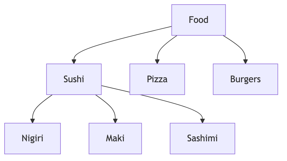
Attributes for “Sushi” might include: cuisine=Japanese, serves_raw_fish=True, typically_contains_rice=True.

Ontologies power:

• Query understanding (“sushi” ∈ Japanese food)

• Faceted search (filter by cuisine, price range, dietary restrictions)

• Recommendation diversity (ensure we cover multiple categories)

8.2 How LLMs help

Traditionally, ontologies were built manually or with rule-based NLP. That doesn’t scale.

LLMs can:

1. Generate category trees

   • Given a list of item names/descriptions, propose a hierarchical category structure.

2. Map items to categories

   • “Assign this product to one of these categories [A, B, C].”

3. Extract structured attributes

   • From textual descriptions, emit JSON with fields like cuisine, price_range, is_vegan_friendly.

4. Discover synonyms and related concepts

   • For semantic expansion: “veggie”, “plant-based”, “vegetarian”.

Pseudo-code for attribute extraction with an LLM (conceptual):

 def extract_attributes(description, llm_client):
     prompt = f”“”
     You are an information extraction system.
     Read the following restaurant description and output JSON with fields:
     cuisine (string), price_level (one of: cheap, medium, expensive),
     vegetarian_friendly (true/false).
 ​
     Description: {description}
     JSON:
     “”“
     response = llm_client.generate(prompt)
     return json.loads(response)

Once you have an ontology:

• Store it in a graph or relational DB.

• Use it in:

  • Query rewriting (“veggie sushi” → add constraint vegetarian_friendly=True).

  • Ranking features (match between query intent and item attributes).

  • Diversification (ensure results cover multiple relevant categories).

---

9. Evaluating Search Results at Scale

You can’t improve what you don’t measure. Search evaluation happens on two axes:

1. Offline metrics: using logged or labeled data.

2. Online metrics: A/B tests on real traffic.

9.1 Offline metrics: NDCG, MRR, Recall@K

Given query q, documents d₁..dₙ with relevance labels rel_i and system ranking:

• DCG@K (Discounted Cumulative Gain):

  \(\text{DCG@K} = \sum_{i=1}^{K} \frac{2^{rel_i} - 1}{\log_2(i+1)}\)

• IDCG@K = DCG of ideal ranking (sort by true relevance).

• NDCG@K:

  \(\text{NDCG@K} = \frac{\text{DCG@K}}{\text{IDCG@K}}\)

• MRR@K (Mean Reciprocal Rank):

  \(\text{RR} = \frac{1}{\text{rank of first relevant item}}\)

• Recall@K: fraction of relevant items retrieved in top‑K.

Simple NDCG@K implementation:

 import numpy as np
 ​
 def dcg_at_k(rels, k):
     rels = np.asarray(rels)[:k]
     gains = 2 ** rels - 1
     discounts = np.log2(np.arange(2, len(rels) + 2))
     return np.sum(gains / discounts)
 ​
 def ndcg_at_k(rels, k):
     ideal = sorted(rels, reverse=True)
     idcg = dcg_at_k(ideal, k)
     if idcg == 0:
         return 0.0
     return dcg_at_k(rels, k) / idcg
 ​
 # Example: model ranking with relevance labels
 rels = [3, 0, 2, 1]  # relevance of items at positions 1..4
 print(ndcg_at_k(rels, k=3))

In a real pipeline:

• Log per‑query predictions and labels.

• Aggregate NDCG@K, MRR@K, Recall@K across queries.

• Compare new models offline before going to A/B testing.

9.2 Online evaluation: A/B tests

Offline metrics have limitations (logging bias, missing labels, etc.). Ultimately, you care about business and user metrics:

• Click-through rate (CTR)

• Conversion rate (purchases, bookings)

• Revenue per session

• Time to first relevant result

• User satisfaction proxies (bounce rate, long dwell time, etc.)

Standard approach:

1. Randomly bucket users into control vs treatment.

2. Control uses baseline search; treatment uses new ranking or retrieval.

3. Run for enough time / users to get statistical power.

4. Check:

   • Primary success metrics (e.g., +X% CTR).

   • Guardrail metrics (latency, errors, crash rate, etc.).

5. Decide whether to ship, iterate, or roll back.

9.3 Evaluation at scale

At scale, you need:

• Aggregation pipelines: compute metrics daily/weekly on billions of log events.

• Monitoring dashboards: track relevance and business KPIs over time.

• Alerting: detect regressions (e.g., NDCG drop due to bug in feature pipeline).

The modeling work (LTR, semantic search, personalization) is only useful if you can reliably measure and monitor impact.

---

10. How NLP Ties Everything Together

NLP is the glue between the components:

• Text embeddings (transformers) → semantic search & LTR features.

• Classification → intent detection, spam detection, query routing.

• Sequence labeling → entity extraction (locations, product types, attributes).

• Generation → query rewriting, summarizing item descriptions, ontology induction.

You don’t need to reinvent NLP; you can:

• Start from pre‑trained models (e.g., BERT variants, sentence transformers).

• Fine‑tune for:

  • Query intent classification.

  • Dual‑encoder retrieval.

  • Sequence labeling for entities.

  • Text‑to‑JSON extraction for ontologies.

---

11. Putting It All Together: A Minimal Search & Ranking Stack

Here’s a summarized architecture combining everything:

This is the ecosystem where:

• Learning‑to‑Rank is the central model.

• Transformers & semantic search power understanding and retrieval.

• Two‑Tower architectures make ANN retrieval scalable.

• NLP underpins query understanding and text features.

• Personalization injects user/context into the ranking.

• LLM‑based ontologies structure the catalog and enrich features.

• Evaluation at scale ensures you’re improving, not just changing.

---

12. Where to Go Next

If you want to see all of this wired together in actual code, I have created a small end‑to‑end project you can run locally: github.com/msaharan/DSAIEngineering/search_and_ranking/search_and_ranking_demo (It links to a specific commit so the code matches the version of the post. Later versions of the code will be available on the main branch.)

It’s a self‑contained, CPU‑friendly mini stack that implements most of the ideas from this post:

• Flow: normalize/understand query → retrieve lexical + semantic candidates → personalize + featurize → train/eval LTR → apply business rules → display results.

• Retrievers: TF‑IDF lexical; optional SentenceTransformer semantic; optional dual‑encoder + ANN stub.

• Ranking: XGBRanker when available, else RandomForest; offline metrics (NDCG/MRR).

• Personalization: simple cuisine/price affinities and user–item bias.

• Rules: vegan boost + cuisine diversity; lightweight ontology‑style enrichment for dietary/category/price hints.

• Data: tiny CSVs in data/ so you can inspect and change everything.

12.1 Run the demo

From the repo root:

 cd search_and_ranking/search_and_ranking_demo
 docker build -t search-ranking-demo .
 docker run --rm -it search-ranking-demo        # semantic + LTR pipeline
 # Lexical-only:
 # docker run --rm -it search-ranking-demo python run_demo.py
 # Dual-encoder + ANN:
 # docker run --rm -it search-ranking-demo python run_demo.py --semantic --dual

The script will, end‑to‑end:

1. Query understanding & intent classification
   Train a TF‑IDF + logistic regression intent classifier on data/query_intents.csv, and add simple query normalization + synonym expansion.

2. Lexical + semantic retrieval
   Build a TF‑IDF lexical retriever, optionally add a SentenceTransformer semantic retriever, and (optionally) a tiny dual‑encoder + ANN stub for semantic candidate generation.

3. Personalization
   Construct simple user profiles (cuisine and price affinities + user–item bias) from data/query_doc_labels.csv, then inject those features into ranking.

4. Learning‑to‑Rank
   Train a ranking model (XGBRanker if available, else RandomForest) on grouped query–item relevance labels and report offline metrics (NDCG, MRR) on held‑out queries.

5. Business rules & ontology‑style enrichment
   Apply lightweight rules such as vegan boosting and cuisine diversity, plus simple ontology‑style enrichment (dietary hints, categories, price range) derived from catalog metadata.

12.2 Suggested experiments

Once you have it running, here are concrete exercises that map back to sections of this post:

1. Lexical vs semantic search (Sections 3–4)

   • Run lexical‑only, then --semantic.

   • Compare which documents surface for ambiguous or “fuzzy” queries.

   • Tweak TF‑IDF and embedding models and see how NDCG/MRR change.

2. Play with query understanding (Section 3)

   • Add new intents and examples to query_intents.csv.

   • Extend the synonym/expansion logic for your own domain.

   • Observe how better query understanding changes candidate sets and ranking.

3. Modify personalization (Section 7)

   • Change how user cuisine/price affinities are computed.

   • Add new user‑level features (e.g., “likes cheap & fast” vs “likes premium & slow”).

   • Watch how different user profiles get different rankings for the same query.

4. Extend the LTR feature set (Section 2)

   • Edit the ranking feature construction to add new signals (e.g., distance, freshness, popularity buckets).

   • Re‑train the model and inspect which features matter most.

5. Experiment with ontology‑style features (Section 8)

   • Enrich catalog.csv with more structured attributes (dietary tags, categories, price bands).

   • Use them in query understanding (e.g., detect “vegan”, “cheap”) and as ranking features.

   • If you have access to an LLM, try auto‑generating these attributes for new items.

6. Change evaluation settings (Section 9)

   • Adjust how train/validation splits are done.

   • Compute NDCG/MRR at different K values and inspect failure cases manually.

Run the demo end-to-end once and you’ll have a working template you can adapt to your own search and recommendation projects.